PYL 105

Part I: Incline acceleration

Motion down an incline is a famous experiment that goes back to Galileo. He was one of the first to understand motion with constant acceleration. For instance, he knew that if the object started from rest then its displacement varied like time squared. Later Newton would relate the accelaration of an object to the net force acting on that object. In the absence of friction and air resistance, theory says that the acceleration down an incline is given by

a = g sin (q)

where q is the angle relative to the horizontal and g is 9.8 m/s² , the acceleration due to gravity. We will attempt to verify this result by the following experiment.

• Connect the Motion Sensor's yellow plug into Digital Channel 1 and its black plug into Digital Channel 2 of the Pasco Signal Interface.
  
  
• Place the Motion Sensor at the top of the incline as shown in the figure below. The direction of the sensor can be varied, make sure it is pointed along the track.
  
  
  
  
  
  
• Set up Data Studio (instructions given in Lab 1), choose Motion Sensor as the device type. Set the Sample Rate (found in the middle on the right hand side of the interface's Experiment Setup) to 20 Hz or 50 Hz. What is "sample rate"?
  
  
• Place the cart 50 cm or more from the Motion Sensor at the top of the incline. This way the first position is in the appropriate range. (A Motion Sensor cannot measure positions that are too close to it; one should always be about 50 cm from it.)
  
  
• Try to coordinate clicking Start and releasing the cart. You may have to eliminate some initial data if you start recording before the cart is released. Try to make sure that there is is nothing between the cart and sensor (like someone's hand) while data is being taken. Stop the cart and stop taking data. Again there may be data at the end that must be eliminated depending on how well this is coordinated.
  
  
• Open Excel and paste the position versus time and velocity versus time data there.
  
  
• We want to analyze only the data when the cart was traveling down the incline without intervention, that is, we do not want data where someone was holding it at the beginning nor do we want data where someone is stopping it at the end.
  
  
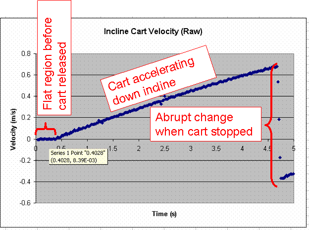
• In order to estimate the release time or the stop time, make a plot of Velocity versus time
  
   
  
  
  
  The flat region indicates the time before the cart is released, the upward sloping region corresponds to the cart accelerating down the track, and the abrupt downward sloping region is where the cart was stopped (before clicking STOP). The pale yellow rectangle was obtained by holding the mouse over a point in Excel.
  
  
• Make an XY Scatter plot of the position versus time data. Fit the plot to a Polynomial of Order 2.  Extract the acceleration.  How?
  
  
• Repeat the experiment at this height twice more.  Then repeat the above process for two other incline angles. Do not try to measure the angles directly. Rather measure the height and hypotenuse of the right triangle formed by the track, block and lab table and use trigonometry.
  
  

  Incline data
  Length of track (  )
  Height ( )	Angle (degrees)	Theoretical Acceleration ( )	Experimental Acceleration Trial 1(  )	Experimental Acceleration Trial 2(  )	Experimental Acceleration Trial 3(  )	Average Acceleration ( )	Standard Deviation ( )	Percent difference

  
  
  
• Do your experimental results agree with the theory? If not, what might account for the discrepancies?
  
  
• Determine the mass of the cart. For one of your angles, add a block (of known mass) to the cart and repeat the measurements.  Add a second block (of known mass) to the cart and repeat the measurements again. From the measurements, determine the experimental acceleration.  How?
  
  

  Incline data: Mass variation
  Cart Mass (kg) (inc. block)	Experimental Acceleration (m/s2) (from graph)	Theoretical Acceleration (m/s2) (from eq.)	Percent error

  
  
  

Part II: The pulley

In the case of the cart on the incline, the cart (in particular its mass) plays a dual role. It is the thing being accelerated, and it is the cause of the acceleration (the gravitational attraction between the mass and that of the earth). Now we will consider a situation in which the cause of the object's acceleration is not its weight.

• Set the track on two of the larger blocks so that it is level.
  
  
• At one end use a universal clamp to secure a pulley at track level.
  
  

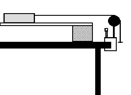
• Place the motion sensor at the other end.  (It is also possible to use a "Smart Pulley" to record the data.) 
  
  
• Tie one end of a string to an empty cart, pass it over a pulley and tie the other end to a hanger. (The string coming from the cart should be horizontal.)
  
  
• Place the cart so that the string is taut and the hanger hangs just below the pulley.
  
  
• Begin recording data and release the cart.
  
  
• Plot velocity versus time, fit the data to a line, and extract the acceleration. Please note that if the hanger hits the floor, the "physics" changes. Before you let the cart go, measure the distance from the floor to the bottom of the hanger and make sure that you stop the cart before it goes that far. Then you can use the kind of observations made in Part I to keep the data up to but not including the time you stopped the cart.
  
  
• Add a block to the cart and repeat the measurements.
  
  
• Add the second block and repeat.
  
  

In the absence of friction and air resistance, theory predicts that

How do your results compare to theory?

Distinguish between the mass-dependence of the accelerations you find for the tilt and for the pulley set-ups.

Part III: Sketching

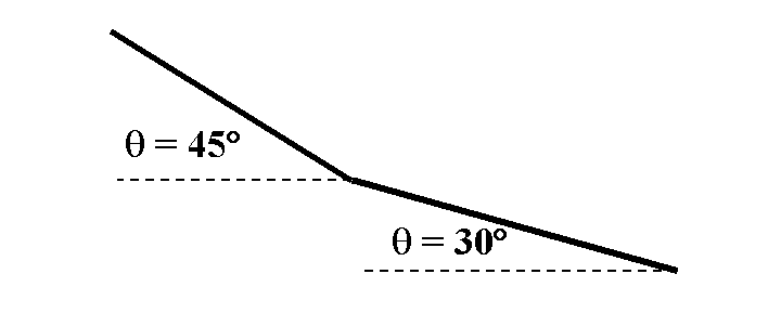
Suppose a mass were sliding along a track like the one shown below.

Sketch a graph of what the velocity-versus-time graph would look like. (Assume the track is two meters long and the bend is in the middle.)