Physics 106 Laboratory: Mass on a Spring

Oscillatory Motion

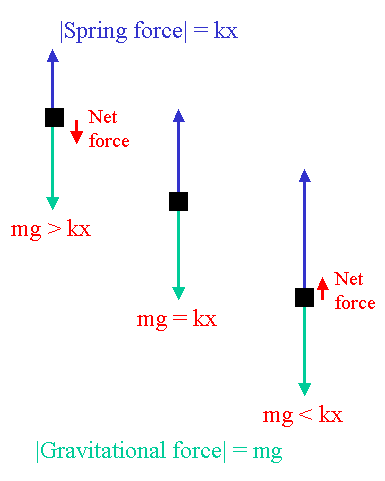
When a mass is hung vertically from a spring, the spring stretches. The force on the mass due to the spring is proportional to the amount the spring is stretched. There is a point at which the spring force and the weight are equal in magnitude but opposite in direction. This point is called the equilibrium position. If the mass is in any other position, there is a net force called the restoring force directed toward the equilibrium position.

The restoring force results in the mass eventually returning to the equilibrium position. The mass, however, picks up some momentum and continues past the equilibrium position causing the same situation as before but on the opposite side of the equilibrium position. The outcome is a repeated motion in which the mass passes through the equilibrium position, turns around, heads back toward the equilibrium position, passes through it, and so on. Such behavior is called oscillatory motion.

(See Chapter 15 in Fundamentals of Physics by Halliday, Resnick and Walker.)

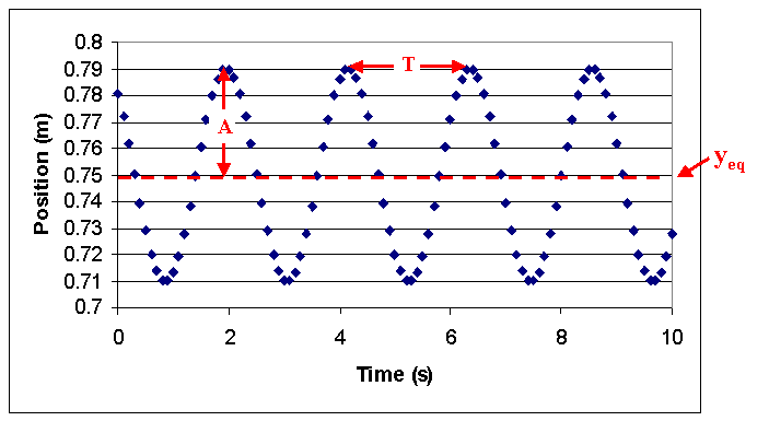
The position of a mass oscillating on a spring can be described by the following equation

y(t) = y_eq + A cos ( 2 π t / T + φ ).

(Compare to eqs. 15-3 and 15-5). The term y_eq is needed in an experiment because the origin is determined by the location of the measuring device, thus the origin cannot be chosen to be the equilibrium position as is typically done in the theoretical account. It is assumed that the argument (the stuff in the parentheses, a.k.a. "the phase") is in radians and NOT in degrees. Note that there are four parameters

• y_eq: the equilibrium position, determines the midpoint of the motion
• A: the amplitude, determines the size the the oscillations, i.e. the maximum displacement from the equilibrium position
• T: the period, determines how much time goes by before the motion begins to repeat itself
• φ: the phase constant, determines the part of the cycle at the beginning, when t=0.

Experiment

• Plug a motion sensor into the PASCO signal interface, the yellow plug should go into Digital Channel 1, the other into Digital Channel 2.
• In Data Studio, double click on the Digital Channel 1 icon and choose Motion sensor. Set the trigger rate to 20 Hz. (You can obtain more data using 50 Hz, but the sensors sometimes have trouble collecting data at that frequency.) For our sensors to work properly, the mass and the sensor should be about 0.5 meters apart.
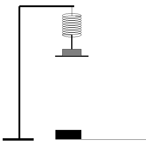
• Place a mass on a spring hanging from a tall ringstand with a motion sensor positioned beneath as shown above. The bar from which the mass hangs should be as far as possible from the motion sensor (i.e. at the top of the ringstand). Do not change its position during the experiment or you will have to retake all of your data.

• Part A. Mass Variations
  • Record the mass, don't forget to include the mass of the hanger. (Enter the sum in the first column of the Mass Variations table in the analysis section.)
  • Set the mass into oscillatory motion (stretch the spring approximately three centimeters and release) and begin recording data. You only need to record a few cycles. Try to ensure that the motion is vertical.
  • Within Data Studio, make a table of the position data. If you do not have a column for Time, then click on the clock button to get the times as well.
  • Copy the columns and paste them into an Excel spreadsheet.
  • Repeat this procedure with several different masses (at least three others, changing the mass by at least 50 g each time).
  • Use a balance to determine the mass of your spring.
  
  
  

  Mass of the spring (       )

  
  
  
• Part B. Amplitude variations
  • Stretch the spring 1 cm from its equilibrium position and release. Use a watch with a second hand (or perhaps a cell phone or an online stopwatch like this one) to record the time required for ten complete oscillations. Divide that number by ten to obtain the period (the time for one complete oscillation) and enter it into the table below.
  • Repeat with amplitudes of 2 cm, 3 cm, 4 cm and 5 cm.
  
  
  
  Amplitude Variations

  Amplitude (cm)	Period (     )
  1
  2
  3
  4
  5

  
  
  

Analysis

1. For each of the masses, plot position versus time [an XY (Scatter) Chart in Excel]. On the same graph, plot a mathematical function that resembles as much as possible your data. Click here for some instructions for this process.
2. You should be able to identify in your function the equilibrium position, the amplitude, period and phase constant associated with this oscillatory motion. Include in your report a table of the masses and this information. The instructions above also tell you how to find the "squares" which provides a numerical way to find the parameters that give the "best fit" -- presumably the fit with the minimum or "least squares".  Perform this step on at least one of your runs.
   
   
   Mass Variations

   Mass (    )	Eq. Pos. (    )	Amplitude (    )	Period (    )	Ph. const. (    )	Squares (    )

   
   
   
3. Plot weight versus y_eq. Recall that to obtain weight in newtons, one multiplies the mass in kilograms by g (9.8 m/s²). Fit this data (i.e. add a trendline) to a straight line. Extract from the fit the force constant of the spring k.
   
   

   Force constant (     )

   
   
   
4. The formula
   
   
   T² = 4 π² m / k
   
   
   comes from squaring both sides of eq. 15-13 (Halliday/Resnick/Walker), which is an idealized equation that assumes the spring is massless. Make a graph of the period squared versus mass (T² versus m) Fit your data to a straight line.
5. The absolute value of x intercept of this graph represents the contribution of the spring's mass to the period. (Note that the constant b in y= m x + b is the y intercept, not the x intercept.) According to your results, what fraction of the spring's mass contributes? How does this compare to the theoretical prediction of 1/3?
   
   

   Mass of spring (     )	x intercept (     )	Fraction	Predicted Fraction	Percent Error
   			1/3

   
   
   
6. Compare your experimental periods to the theoretical values

   T = 2 π ( m / k )^1/2.

   and to a corrected theory that takes into account the effect of the spring's mass

   T_cor = 2 π [ (m + 0.333 m_spring) / k ]^1/2.

   Exper.     Period (    )	Theor.     Period (    )	Percent Difference (    )	Corrected Theor. Period (    )	Percent Difference (    )

   
   
   
7. Plot period versus mass (using the data in which the mass was varied -- Part A) and period versus amplitude (using the data in which the amplitude was varied but mass held fixed -- Part B). Make sure that the two plots have the same scale on the y axis. (If you need to change the scale on one or both, right click on the numbers along the y axis and choose Format Axis, select the Scale tab (Excel 2003) or Axis Option (Excel 2007), and enter values in the Minimum and Maximum textboxes. The Auto checkbox/radiobutton should not be checked.) What can you conclude from this comparison of period's dependences on mass and amplitude?