Conversations on Nonequilibrium Physics With an Extraterrestrial

Nonequilibrium systems come in many varieties, and a number of not−yet−reconciled mathematical approaches can be applied to them.

A couple of years ago I was visited by a Slimy Galactic Superoctopus−−a being from outer space who, for the occasion, had taken on a female human appearance. Were it not for her spaceship in my garden and a few other details, I would have said she was just a pleasant young woman, very intelligent and pretty. She told me her name was Pallas. She had been writing a galactic PhD thesis on the nature of human mathematics, and we had long discussions on that and other topics.¹ Then Pallas had to pass her exams and she disappeared into the darkness of space. I had little hope of seeing her again. But once more, her tall, white, silent spaceship stood in my garden, and when we met at the garden door, it was as if she had never been away.

While we were strolling along one of the paths we had walked before, she said, "I would like to understand your interests in mathematical physics."

Figure 1

"Currently I am looking at problems in statistical mechanics, nonequilibrium to be specific," I answered. "It's an area of rapid progress in which scientists have finally gained some fundamental understanding of situations far from equilibrium. Many biological processes, by the way, are in that category." (See figure 1.)

"Statistical mechanics," I continued, "attempts to explain the macroscopic properties of matter in terms of the interactions of its microscopic constituents. To be precise, one starts with a mathematical description of the time evolution of a system of many particles−−molecules for example. The evolution is deterministic, defined by a Hamiltonian H that may be classical or quantum. I shall now squeeze more than a century of work on equilibrium and nonequilibrium statistical mechanics into a few words. Ready?"

"Yes. Please go on."

"Statistical mechanics was developed at the end of the 19th century by, among others, James Clerk Maxwell, Ludwig Boltzmann, and Josiah Willard Gibbs. Equilibrium statistical mechanics is concerned with certain states of matter that appear macroscopically at rest, in equilibrium, and that are microscopically a superposition of states i, with probabilities p_i. A simple example is that of a quantum spin system, a type of quantum system with a finite−dimensional Hilbert space. Let E₁, . . ., E_n be the eigenvalues of the Hamiltonian H, and express temperature in units of energy. An equilibrium state at inverse temperature β is then defined by associating with each eigenvalue E_i a probability p_i = exp(−βE_i)/Σ_j exp(−βE_j), obtained by normalizing the so−called Boltzmann factor exp(−βE_i). For more general systems, the set of states will be infinite and sums may be replaced by integrals.

"If the Hamiltonian describes particles that repel each other at short distances and have negligible interaction at large distances, then an asymptotic 'thermodynamic limit' exists in which the volume and number of particles tend to infinity at fixed density and temperature. Or, instead of fixing the temperature, one can fix the energy density: The two types of description are equivalent. In favorable cases, one can study phase transitions, the critical points, and so forth. Difficult problems remain, though, such as proving the existence of crystal phases, but the successes of equilibrium statistical mechanics during the 20th century were stupendous.

"After the foundations were laid in the 19th century, equilibrium statistical mechanics developed slowly at first, then rapidly. The 19th century also saw the development of basic ideas of nonequilibrium statistical mechanics. Boltzmann showed how entropy, which measures the amount of microscopic randomness compatible with a macroscopic description, could statistically only increase with time. The philosophically correct views of Boltzmann, however, did not lead to a simple, general, useful prescription that could be systematically used to attack nonequilibrium problems." (For a modern description of Boltzmann's ideas, see the article by Joel Lebowitz in Physics Today, September 1993, page 32.)

"Note that instead of nonequilibrium," I continued, "people also speak of dissipation or irreversibility. The three terms refer to different aspects of the same thing: When a system is outside of equilibrium, it dissipates energy as heat, and that happens with an irreversible increase of the entropy. Mechanical, chemical, and electrical energy may all be dissipated in irreversible processes."

All the time I had been describing statistical mechanics, Pallas had been smiling and had remained silent. Now she said, "Can you tell me the real reason why nonequilibrium is harder than equilibrium? And can you give me an example of both?"

I answered, "In the description that I just gave, equilibrium theory starts with the Boltzmann factors, exp (−βE_i): The dynamics−−that is, time evolution−−is eliminated. All one needs to know are the energies of the various states. In nonequilibrium problems, the dynamics cannot be forgotten. Consider specific heat and heat resistance. For specific heat, one asks how much heat needs to be put in a lump of matter to increase its temperature by one degree. For heat resistance, one asks what temperature difference needs to be put across a lump of matter to force a unit of energy to pass through the lump per unit time. The two problems may not sound very different, but the first is equilibrium, does not involve dynamics, and is relatively easy. The second is nonequilibrium, involves dynamics, and is difficult."

By the time she asked her next question, Pallas's smile had definitely become mischievous.

"Because dynamics is important for questions of nonequilibrium, wouldn't you start with simple dynamics that you can understand in detail?"

"A natural idea, indeed, is to study the heat resistance of a chain of harmonically coupled harmonic oscillators," I replied. "This system is completely integrable, the Hamiltonian is quadratic, and everything can be computed explicitly. But the results are pathological: The resistance is not asymptotically proportional to the length of the chain as one would expect on physical grounds.² Completely integrable systems may be all right for easy computation, but they are not what we need to study nonequilibrium systems. If you think about it, completely integrable dynamics is exceptional, and we should consider a type of dynamics that is common rather than exceptional.

"Chaotic dynamics is a natural choice. That somewhat loose term describes time evolution with sensitive
dependence on initial conditions. Thus, a small change δx(0) in the initial condition x(0) typically gives δx(t) ≈ δx(0) exp(λt), with the so−called Lyapunov exponent λ > 0. There exist mathematical arguments that most dynamical systems are chaotic in some sense. So it is reasonable to assume chaos for the microscopic dynamics−−both for equilibrium and nonequilibrium situations. But while chaotic dynamics is common, such behavior does not cover all situations of physical interest. In fact, Andrei Kolmogorov, Vladimir Arnold, and Jürgen Moser have described distinctly nonchaotic behavior that is relevant to some situations in statistical mechanics."³

Pallas interrupted. "I see a difficulty. You have to base the study of nonequilibrium systems on a mathematical understanding of dynamics, but you don't know what general dynamical systems look like. For thousands of years, scientists throughout the galaxy have tried to understand general dynamical systems, and it is not an easy problem. To avoid getting mired in mathematical questions beyond human capabilities, perhaps you should stay closer to physics."

I get upset when Pallas implies that the human brain is a rather limited intellectual tool, better suited to hunting rabbits than doing mathematics, and that Slimy Galactic Superoctopuses are mathematically quite superior to us. But keeping the physics in mind is certainly a good point.

"The Newtonian gravitational force," I noted, "does not lead to thermodynamic equilibrium because it is attracting and also because it is long range. Water left in a bottle outside the house in winter may remain liquid well below 0°C. It is in a metastable state, but will freeze rapidly when one bangs the bottle. When a piece of iron is placed in an oscillating magnetic field, it produces heat, and the magnetization of the iron depends on previous values of the magnetic field, not just the instantaneous value. That behavior is called hysteresis. A temperature difference imposed between two faces of a lump of matter may lead to a nonequilibrium steady state, or NESS, in which heat is transported from the warm to the cold face. Another kind of NESS can arise when reacting chemicals are pumped into a tank and stirred, and excess mixture is able to flow out, although sometimes for such systems, one gets oscillations. Gravitational collapse, metastability, magnetic hysteresis, transport, and chemical reactions are all examples of nonequilibrium phenomena [see figure 2]. Since the physics of those examples is rather different, I'll concentrate on NESSs, and allow both transport and chemical reactions.

Figure 2

"Spatial structure is important for transport phenomena, in which heat, chemical concentration, or momentum carried by a viscous fluid is transported through matter. Typically, the transport phenomena are locally close to equilibrium. The matter in which transport occurs appears close to an equilibrium state at some temperature, pressure, and so forth when one observes on a small but still macroscopic scale, say 10⁻² mm. Note that the macroscopic equations for transport, such as the heat and diffusion equations or the Navier− Stokes equation, usually contain a Laplace operator −² with an appropriate coefficient, called a transport coefficient. The Laplace operator describes diffusion of heat, concentration, or momentum. One might say that in transport phenomena, dissipation is of diffusive nature. Chemical reactions, which are far from equilibrium, normally have no macroscopic spatial structure." Later on in our stroll, I told Pallas a bit more about transport coefficients and introduced her to some important 20th−century contributors to nonequilibrium statistical mechanics. (See box 1.)

"Physics," I informed Pallas, "seems to be in a foundational period for nonequilibrium statistical mechanics, with an explosion of very interesting and sophisticated work. Assumptions vary−−classical or quantum theory, deterministic or stochastic dynamics, finite or infinite number of degrees of freedom. The relations between the various approaches have not yet been worked out.

"When a system is out of equilibrium, it dissipates energy into heat. Therefore, for it to reach a steady state, the system needs a thermostat to cool it. One useful idealization of such a system has a finite number of degrees of freedom subject to non−Hamiltonian forces. William Hoover and Dennis Evans modified the Hamiltonian equation

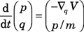(1a)

to obtain

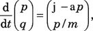(1b)

where ξ is no longer assumed to be a gradient, and α = ξ(q) ⋅ p/p². For simplicity, I'm expressing quantities as if they were one−dimensional, but my discussion is general and applies to phase space of arbitrary even dimension.

"The term −αp implements the so−called isokinetic thermostat and ensures that the time evolution preserves the kinetic energy p²/2m. Note that in the lab, a thermostat usually cools a system at its boundary. By contrast, the isokinetic thermostat cools the bulk. That is physically somewhat different, but not unreasonable, and very convenient for mathematical discussion."⁴

"Isn't it distressing," Pallas interrupted, "that you abandon Hamiltonian mechanics? Is it necessary?"

"A possible way to look at it," I replied, "is that one starts with an infinite system because an infinite reservoir acts as a thermostat. Then one integrates away the coordinates of the reservoir and is left with a finite non−Hamiltonian system. Because of the non−Hamiltonian dynamics, the volume in phase space is no longer conserved. As I'll explain soon, that volume contraction can be identified with entropy production."

"Integrate away the reservoir," said Pallas. "That is easier said than done."

"Exactly. It can be done formally, but we are still waiting for a serious treatment. Note that Pierre Gaspard has a purely Hamiltonian approach based on diffusion. His work begs to be connected to other approaches."

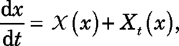
"A few years ago," I continued, "Giovanni Gallavotti made me aware that various ideas present in the literature, when put together, amount to a theory of NESSs in which one does not assume closeness to equilibrium. That observation was used by Gallavotti and Eddie Cohen to prove their important fluctuation theorem.⁵ But before I go into that, let me outline a five−point general theoretical framework for NESSs. It's basically what Gallavotti told me, with the addition of the linear−response formula."

Deterministic dynamics. "I assume that the nonequilibrium time evolution is given by

(2)

where I have further abbreviated the notation by writing x instead of (p, q) for a point in phase space with fixed kinetic energy. The symbol Χ denotes a vector field, such as appeared on the right−hand side of equation 1b.

"The solution to equation 2 may be expressed in the form x(t) = f^tx(0), which defines a nonlinear evolution operator f^t. It is often desirable to impose time−reversal symmetry. In the case of equation 1b for example, that symmetry means the equation remains valid when (t, p) goes to (−t, −p) while q and ξ are unchanged."

Chaos. "Earlier I noted that chaotic time evolution is natural in both equilibrium and nonequilibrium systems. A chaotic time evolution stretches distances in some directions of phase space−−that stretching leads to the sensitive dependence on initial conditions−−and it contracts distances in other directions. Gallavotti and Cohen imposed a chaotic hypothesis in the mathematically precise sense of uniform hyperbolicity.⁶ They also assume that time is a discrete variable. Uniform hyperbolicity is perhaps too strong physically so, for now, I'll remain vague about just what I mean by chaotic dynamics and make further assumptions as I go."

A measure for a NESS. "Since the time evolution described by equation 2 is not Hamiltonian, it will not, in general, preserve the phase−space volume m, no matter how that volume is defined. (Think of dp dq if you want to have a specific example for m.) In light of the nonconservation of volume, I'll consider more general measures ρ with respect to which any continuous function A has an integral −− ρ(dx) A(x). The measure ρ may be singular, as is the case for the Dirac delta measure.

"For a chaotic system, many measures are invariant under time evolution. Which one is the best choice to describe a NESS? Suppose that the time averages of continuous functions A are given by a measure ρ in the sense that

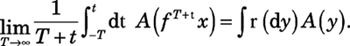(eqn 3)

Despite appearances, it is often the case that the limit in the left−hand side is independent of time t and phase−space coordinate x. Thus, for a large set of initial conditions−−in particular, a set for which the measure m gives a nonzero volume−−measures like ρ implement time averages and are physically natural choices for a NESS. Called SRB measures, they were introduced by Yakov Sinai, Rufus Bowen, and me, then discussed more generally by Jean−Marie Strelcyn, François Ledrappier, and Lai−Sang Young. As early as the 1970s, it appeared that such measures might be appropriate for describing nonequilibrium systems, but the idea could be implemented only after deterministic thermostats were introduced.

Box 2

"One may define a NESS in terms of an SRB measure ρ; in particular, one assumes that such a measure exists. Completely integrable systems do not have SRB measures as just described, but an SRB measure is uniquely determined when the chaotic hypothesis of Gallavotti and Cohen is satisfied. Note that the introduction of the measure breaks time−reversal symmetry because I let the time τ go to −∞, not +∞."

  At this point, Pallas voiced a request: "I wonder if you might draw a picture to illustrate the stretching of phase−space dimensions and the singular nature of the SRB measure."

I found a napkin and sketched the figure that appears in box 2.

Entropy production as volume contraction. "The average rate of entropy production in the NESS compatible with ρ is

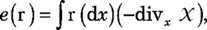(4)

where the divergence is computed with respect to the volume element m. Invariance of ρ under time evolution implies that any choice of m gives the same value for e(ρ).

"One can obtain equation 4 by a formal calculation based on the Gibbs expression −∫{m(dx)g(x) ln g(x)} for the entropy corresponding to a probability distribution g(x)m(dx). A key technical element in the calculation is that [as discussed in box 2] the appropriately normalized volume m evolves to the SRB measure ρ as time becomes infinite. The relation between equation 4 and the Gibbs expression was apparently first noted by Ladislav Andrey.⁷ The general relation between entropy production rate and phase−space volume contraction is still debated, but equation 4 appears to be correct when one has a deterministic thermostat.

"If ρ is an SRB measure, one can show that e(ρ) ≥ 0; for the interesting case of dissipation, e(ρ) > 0. The positivity of e(ρ) is tied to the fact that introducing the SRB measure breaks time−reversal symmetry. In the Hamiltonian case, time evolution preserves phase−space volume and divΧ = 0."

Linear response. "Statistical mechanics aims to compute the response of a system to an external action. The specific heat, which describes how a system reacts to external heat input, is an example. To include an external action, one can modify the time evolution, equation 2, to obtain

(5a)

where X_t is a small perturbation of Χ that may depend on the time t. Given such a perturbation, the SRB state ρ would be replaced by ρ + δ_tρ. A simple formal calculation yields

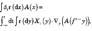(5b)

where f^t is the evolution operator for the unperturbed time evolution. In the linear−response formula, equation 5b, A is assumed to be differentiable rather than just continuous. The formula can be rigorously proved under the assumption of uniform hyperbolicity−−the chaotic hypothesis of Gallavotti and Cohen." For further discussion see references 6 and 8.

"So," said Pallas, "you claim that the five points you just listed constitute a theory of nonequilibrium? In what sense?"

"In the sense that, given a suitable physical question, one can in principle write an answer. There may be integrals, limits, and so forth that one cannot explicitly perform, but such difficulties also accompanied equilibrium statistical mechanics after Boltzmann and Gibbs, and the 'close to equilibrium' theory developed by Lars Onsager, Mel Green, and Ryogo Kubo around 1950. In fact, the theory I just outlined is an extension of that close−to−equilibrium work, with closeness to equilibrium not assumed. Now I want to discuss briefly two physically significant examples.

"First is the remarkable Gallavotti−Cohen fluctuation theorem.⁵ Their formula, which has no adjustable parameters, gives the fluctuations in the rate of entropy production for a NESS. It has been rigorously proved, given the chaotic hypothesis, and thus adds a new dimension to earlier, more formal results.⁹ The chaotic hypothesis is overly restrictive, and it is remarkable that it gives the right answer: Apparently, dynamical systems associated with statistical mechanics often behave as if they were uniformly hyperbolic.

Figure 3

"My second example is also related to fluctuations. Consider the fluctuation−dissipation theorem, which is valid close to equilibrium. The theorem relates the spontaneous fluctuations of a system to the response of the system to an external action. The physical idea is that in order to know how a system reacts to a kick, one might as well wait until the system has a fluctuation equivalent to the result of that kick. Then one can see what happens. A special case of the fluctuation−dissipation theorem is the Green−Kubo formula, which expresses transport coefficients in terms of time correlation functions.

"Efforts to extend the fluctuation−dissipation theorem far from equilibrium would be expected to fail in general. Indeed, in the five−point theory I laid out, the NESS lives on a phase−space attractor that is generally fractal. One could kick the system to a point outside of the attractor, but such a point cannot be visited by spontaneous fluctuations. Therefore, fluctuations cannot reveal how the system reacts to such a kick. One might, though, expect that the theorem could be partially extended to allow for kicks that keep the system on the attractor."^6,8

Pallas interrupted me. "I can see a couple of big problems that you have not addressed. One is that statistical mechanics is generally about large systems, systems with many degrees of freedom. How do you take the limit?"

"That indeed may be a formidable problem," I admitted. "After all, in some cases a large system will undergo oscillations in time rather than behave as a steady state! My inclination is to postpone the study of the large−system limit: Since it is feasible to analyze the nonequilibrium properties of finite systems−−as Gibbs did for their equilibrium properties−−it seems a good idea to start there. That may not answer all questions, but it advances nonequilibrium statistical mechanics to the point equilibrium had reached after Gibbs."

But Pallas saw another big problem. She noted that varying the parameters of a physical system amounts to changing the time evolution, equation 2, which typically produces many changes of behavior, so−called bifurcations. The linear−response formula, equation 5b, assumes smooth dependence on parameters, and that's unlikely to hold. So the integration over time in that formula may be divergent.

"In fact," I told her, "the same problem arises for the Green−Kubo formula close to equilibrium. Nico van Kampen has remarked that, in situations in which one typically applies Green−Kubo, one would expect the linear−response formula to be mathematically valid only for unphysically small perturbations of equilibrium.¹⁰ How serious are these objections? Consider the following three facts. First, Green−Kubo works. That is, it is consistent with experiments and computer simulations with large systems. Second, the linear−response formula can be proved for uniformly hyperbolic systems, including those considered by Gallavotti and Cohen. Third, bifurcations messing up Green−Kubo are seen in systems that are small and nonuniformly hyperbolic.

"Theorists believe that most physical systems are not uniformly hyperbolic and that they would exhibit many bifurcations. Nonetheless, typical large systems seem to behave as if they were uniformly hyperbolic. One would certainly like to understand why that is the case.

"When we have more time, I can explain a variety of technical results that really convince me that we are on the right track to understanding nonequilibrium physics."¹¹

With a somewhat ironic smile, Pallas said, "On my next visit to Earth, I will check with you to see if ideas on nonequilibrium statistical mechanics have progressed in the direction you indicated. But for now let us leave this discussion. Would you like to listen to some music?"

"Well . . . there are relations between nonequilibrium and music, but is that the real reason you ask?"

"It is something else. You know how unnatural the tampered scale is−−brutally cut by human musicians into 12 equal half−tones, every interval slightly wrong. Because of your imperfect human hearing, you do not realize it, but the result is truly abominable. And the funny thing is that I have come to enjoy it! Isn't that very perverse?"

"Tempered scale," I said weakly, "not tampered. And Johann Sebastian Bach is neither truly abominable nor very perverse." This time I was really upset.

But Pallas just smiled sweetly. "Ready to listen to some preludes and fugues from the Well−Tempered Clavier?"

This article is a reworking of the Shih−I Pai lecture I gave at the University of Maryland, College Park, in April 2003.

© 2004 American Institute of Physics