PYL 105: Lab 1

Introduction to graphing, scaling and the Pasco Interface

In physics, we explore the relationships among properties of light and matter (physical quantities) by comparing them to mathematical relationships, generally expressed in the form of equations. In order to do this we need

1. The experiment: apparatus designed to measure the desired quantities;
2. The theory: a proposed mathematical relationship between variables representing the quantities;
3. The comparison: an analysis of whether or not the data from the experiment and the equation from the theory agree with one another.

These steps are crucial to the "Scientific Method." (Newtonian Physics, p. 15) Of course, physics is more just than matching up data with equations, the theory should explain what is happening in the experiment, relate it to other experiments, and ultimately suggest new experiments and make predictions about their outcomes.

If one finds disagreement between theory and experiment, then there must be a flaw or shortcoming in the experiment, the theory or the analysis. While the theories studied in this class are fairly well established, the results are often over-simplified. For example, they often neglect the effect of friction or air resistance.

To model some of the situations that occur when we are comparing data and theory, let us imagine an experiment in which we measure the radii and areas of circles. In this case the theory is encapsulated in the equation: A = pr². A very accurate and precise experiment might yield data like the following

Radius (cm)	Area (cm^2)
0.210741	0.139523
0.370969	0.432341
1.468089	6.771024
1.506797	7.132793
1.799232	10.170080
2.374442	17.712218
2.393784	18.001963
5.403330	91.721846
7.102157	158.463910
8.212887	211.905158

Note that the units (cm and cm²) of the measured quantities are provided in the column labels! We use the meter as our standard unit of length. A centimeter is 10^-2 m. (Newtonian Physics, pp. 22-27)

Now assume we performed the same experiment with less precise instruments. (The data below was obtained simply by rounding the data above.)

Measured Radius (cm)	Measured Area (cm^2)	Theoretical Area (cm^2) A= pr^2	Deviation (cm^2)	Percent Error
0.2	0.1
0.4	0.4
1.5	6.8
1.5	7.1
1.8	10.2
2.4	17.7
2.4	18.0
5.4	91.7
7.1	158.5
8.2	211.9

Consider the radii above to be precise and calculate the corresponding theoretical areas (A = pr²) and put them in the third column. Then subtract the third column from the second and place that result in the fourth column. Finally divide the fourth column by the theoretical value (third column) and multiply by 100 to find the percent error, place that in the fifth column.

Next suppose that the apparatus for measuring areas was miscalibrated. We will model this by adding 0.2 to all of the above areas, giving

Measured Radius (cm)	Measured Area (cm^2)	Theoretical Area (cm^2) A= pr^2	Deviation (cm^2)	Percent Error
0.2	0.3
0.4	0.6
1.5	7.0
1.5	7.3
1.8	10.4
2.4	17.9
2.4	18.2
5.4	91.9
7.1	158.7
8.2	212.1

Perform the same calculations as before on this data.

The "error" -- the difference between the actual measurement and an ideal, perfect measurement -- comes in two varieties:

• Systematic: A systematic error follows a pattern; the same deviation would occur if you repeated the measurement provided you use the same equipment and same technique. Thus the deviations associated with it can be predicted. Measurements with little or no systematic error are said to be "accurate."
• Random: A random error shows no recognizable pattern; the deviations associated with it are as likely to be positive as negative. Random errors are dealt with using statistical analysis. Measurements with little or no random error are said to be "precise."

In the example above, the calibration error was systematic, the same effect occurred in each measurement. On the other hand, the rounding errors were random; one was just as likely to round up as to round down. In most cases we have a combination of systematic and random error. When we have luxury of a precise theoretical prediction, we can look at the average of the deviations. Since random-error deviations are as likely to be positive as negative, the average deviation should be zero or close thereto.

Sometimes a theory predicts not a definite equation but just a mathematical form. For instance, instead of predicting precisely

A = pr²

a theory may predict only the power-law form

A = Cr^a

leaving the parameters C (the coefficient) and a (the power) to be determined by the experiment. When you are comparing data to a form rather than a precise equation, you choose the parameters that make for the best comparison. This process is referred to as "fitting the data;" it provides one with the previously unknown parameters and simultaneously compares the data to the mathematical form.

We can visualize the comparison of the experimental data and the fit to theory by placing them on the same graph. Note that in order to distinguish the data from the fit, it is conventional to plot the data as unconnected points, and a fit as a line. A good fit will pass close to or indeed go through as many points as possible. Sometimes we see what we want to see, so it is useful to have a quantitative measure of whether a fit is good. One such measure is called the R² value. An R² value near one indicates a good fit.

Even when theory predicts a precise equation, it is a good test of the theory to adopt only the mathematical form of the equation and fit the data to it. When the data matches the power-law form shown above, the data is said to exhibit "scaling behavior." (Newtonian Physics, pp. 37-46) Many of the relationships we will consider in this course fall into this category.

Let us see whether the data with the rounding and calibration errors still obeys a scaling law. To do this we graph the data and fit it to a power law. There can be some subtle issues in fitting, but for the most part finding the best fit is a straightforward though tedious procedure. Fortunately, Excel has built in the fitting procedure to a number of standard functional forms -- including power laws.

• If you are using Internet Explorer, you can copy the data above and paste it into Excel. If you are using Netscape, it may not copy properly. Enter the data into Excel or switch to Internet Explorer.
• Plot Area versus radius for the above data in an XY Scatter graph and fit it to a power law. The default Type (mathematical form) is a straight line; make sure you change the Type to Power.
• If you have never made an XY Scatter graph using Excel or if you need a refresher, follow these instructions. (We will be doing this procedure a lot, learn it!)

Sometimes an experiment is done for which there is no theory or perhaps there are two competing theories. Determine which of the functional forms available in Excel fits best.

X	Y
0.2	0.46
0.4	1.10
1.5	5.29
1.5	5.32
1.8	6.98
2.4	10.62
2.4	10.71
5.4	40.01
7.1	64.69
8.2	83.78

How did you make you determination?

The Trendline Types that Excel has available are very useful, but we will occasionally need other functions. One standard function not available is the sine function. Plot the following data.

X	sin(X)
0.0	0.00000
0.3	0.29552
0.6	0.564642
0.9	0.783327
1.2	0.932039
1.5	0.997495
1.8	0.973848
2.1	0.863209
2.4	0.675463
2.7	0.42738
3.0	0.14112
3.3	-0.15775
3.6	-0.44252
3.9	-0.68777
4.2	-0.87158
4.5	-0.97753
4.8	-0.99616
5.1	-0.92581
5.4	-0.77276
5.7	-0.55069
6.0	-0.27942
6.3	0.016814
6.6	0.311541
6.9	0.57844

The Pendulum

Let us put some of these graphing skills to use in an actual experiment.

A simple pendulum is a mass hanging from a string. A pendulum is said to exhibit periodic motion, that is, its motion repeats itself, taking the same amount of time each time. We call the time the pendulum takes before it starts repeating itself the period T. We want to study the effect on the period of varying

• the mass of the bob
• the length of the string

You should make sure that when varying one parameter, the others are held fixed.

For the Pasco Scientific Interface to work properly, it should have been turned on BEFORE your computer. If this was not the case, log off, turn the computer off, make sure the interface is on, then turn the computer on and log on.

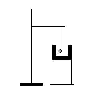
• Plug a photogate (U-shaped apparatus shown below) into Digital Channel 1 of the interface.

• Open up Science Workshop, you will find it under Start/Programs/Physics/Science Workshop/Science Workshop.
• Drag the digital plug icon into the Digital Channel 1 icon and choose Photogate & Pendulum from the menu.
• Using a ringstand, clamps, a mass, some string, and so on, set up a pendulum as shown above.
• We will use the cylindrical shaped masses as our bobs.
• Make sure that as the bob is moving, it passes through the center of the U-shaped part of the photogate.
• Initiate the pendulum's motion, record data for a few periods.
• Drag a table into Digital Channel 1 and choose Period from the menu.
• If you click on the button with a S, then the average and standard deviation (spread in the data) will be displayed. If the data is not consistent (little to no spread), then retake the data.

Vary the bob mass.

• Tie bobs of different masses to your the end of your string.
• To the best of your ability, make sure that the distance between the length of the string from the crossbar to the center of mass of the bob remains fixed.
• Make sure you release the bob from the same initial angle; you may want to use a protractor.
• Record the masses and the periods for four different bobs.

· Vary the pendulum length.

• Vary the length of the pendulum. To ensure a substantial range of variation, your smallest length should be at most half as long as your longest length.
• Keep the mass and initial angle fixed.
• Record the lengths and periods for five different lengths.

• Plot the period versus mass. What kind of dependence if any do you see?
• Plot the period versus length. Fit it to a power law. What power do you find? According to theory

T = 2.01 L^1/2

where T is the period measured in seconds and L is the length measured in meters. (College Physics, p. 129) Do your results agree with theory?